Simulating climate, air pollution, and nitrogen

Modeling in climate science is a complicated topic. These models have to do very difficult tasks - modeling climate, and are expected to inform future directions of climate change, air pollution, nitrogen deposition, and other questions that have huge consequences. The only way to deal with systems this complex is simulation. You attempt to encapsulate physics and chemistry into equations, you approximate those equations on a computer, and you run controlled experiments that would be impossible to run on the actual planet. In this article, I will try to learn and explain some of the necessary components for simulating environment.

A good starting point is to describe what these kinds of simulator actually are. The simulator stores a state, advances it forward in time, and produces new states. These states can be whatever, but in the case of environment, they consist of things like winds, temperature, humidity, pressure, clouds, and chemical concentrations.

The simulations consist of different groups of values: initial conditions specify the starting state, usually assembled from observations and previous model fields. Boundary conditions describe what enters or constrains the domain, such as sea-surface conditions, or land-surface properties. External forcing is a way to push the model using input values, such as greenhouse gas concentrations and aerosol forcing relevant for many climate experiments. Of course some things aren't certain, so many things have to be guessed and estimated (chemical mechanisms, tiny level turbulence or cloud physics). This is important, as these decisions can add up and lead to different results. Here in the Netherlands, the AERIUS Calculator handbook is explicit about the decisions and technical difficulty of climate modeling.

On a large scale, the simulation is an equation that maps a state to a new state - like an equation that calculates what happens next. If \(x(t)\) is the full model state, then the continuous time evolution is

where \(u\) stands for prescribed inputs like emissions and forcing, and \(\theta\) stands for parameters inside closures and subgrid schemes. A computer cannot evolve these kind of equations exactly, so the model replaces it with a discrete model that only updates at small timesteps \(\Delta t\),

where \(\mathcal{M}_{\Delta t}\) is the time-advance operator that takes into account all dynamics. When we write down the equations like this, we can see that in principle it is simple, but in reality, there's a lot of things to take into account for these parameters.

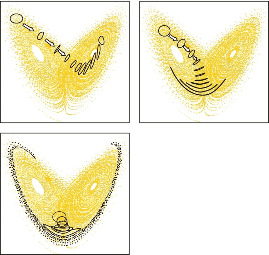
The atmosphere is a nonlinear chaotic system, so small differences in starting conditions \(x_0\), small differences in prescribed inputs \(u\), and small differences in parameters \(\theta\) can grow as the model is stepped forward by \(\mathcal{M}_{\Delta t}\). That sensitivity limits what a single simulation trajectory can mean, especially if you get into the small-scale effects, so modern practice treats one run as just a realization rather than the realization. The solution is to run an ensemble: they repeat the simulation many times with slightly different initial conditions, sometimes perturbed parameters, and sometimes alternative model configurations, then summarize the distribution through its mean, spread, and tail behavior.

For air pollution and nitrogen, a large part of \(F\) consists of chemistry and movement of molecules. If \(c(\mathbf{r},t)\) is the concentration of a species, a common conceptual form is

where \(\mathbf{v}\) is wind, \(K\) is a turbulent mixing term (diffusion), \(S\) includes emissions and chemical production, and \(R\) includes chemical loss and removal, for instance through rain. Since these steps are hard to calculate and estimate, different models make different choices about how detailed \(S\) and \(R\) should be.

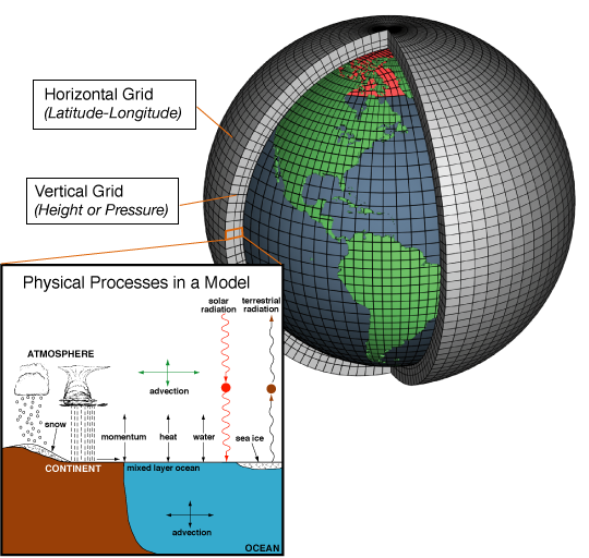
Time is not the only thing we have to break into small pieces to solve the equation. Space is also pretty much continuous in real life, and we have to break it up into finite-volumes (somewhat akin to Finite element method, but nowadays models specifically use spectral element method).

The largest block of assumptions are in the processes that are smaller than the grids we break space and time into. Clouds, convection, and atmospheric chemistry cannot be resolved explicitly at typical climate-model grid spacing, so models use parameterizations: compact rules for the average effect of processes. Parameterizations are one of the main reasons different models disagree on regional rain, or extreme-events. How can we try to improve this?

• One strategy is to just increase resolution by making the grids smaller, or by changing the local resolution where needed. Imagine using a smaller grid for a densely populated area, or a particularly dangerous area.
• The second strategy is to build stochastic parameterizations that try to capture the variability of these small processes. While this doesn't technically give you the answer, on average you will get a better representation of the results. Similar to have we discussed ensemble simulation, this allows variation during the simulation to not get fixated on just a solution.
• The third strategy is hybrid modeling, where machine learning tries to help fill in some of the blanks. This approach is gaining popularity and in my opinion has a lot of potential. The benefits of this kind of approach is the potential to help improve accuracy, reduce energy use, and increase speed.

All-in all, climate modeling requires complex computation, accurate guesses and descriptions of reality, and it can be a wonder we have anything working at all. The future for climate is bright, though, as I think machine learning is at a prime position to help solve many of the problems. Google Deepmind agrees with me, and has already started making progress on the questions at hand.